Understanding the HydraCALC Printout

The standard HydraCALC printout conforms to NFPA13 specifications. There are alternate printout options available, but what follows are the standard sheets and their explanation.

Cover Sheet

The Cover Sheet begins the submittal calculations. It consists of a logo, your company information (if so configured) and some pertinent calculation information.

The version number of HydraCALC used to produce the calculation is at bottom.

The logo of this sheet can be changed as explained in this earlier section: Setting Up Your Own Company Cover Sheet

The company name and address can be changed as detailed in this earlier section: Altering Company Information

The bottom section is automatically filled out and gets its values from the Information Sheet, except for the last item - the Data File. That is the file name of the calculation.

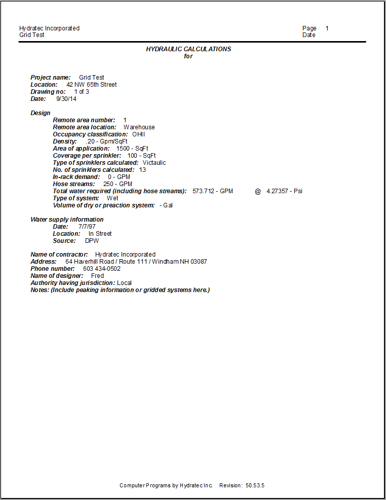
Summary (Information) Sheet

The Summary Sheet is based entirely on the Information Sheet you created in HydraCALC, if you in fact created one.

Water Supply (Hydraulic Graph)

The Hydraulic Graph sheet is generated from the data that was entered using the Water Supplies command along with data entered into the job itself. It shows curves based on city supplies and pumps, if any. This page prints in landscape mode.

Types of Hydraulic Graphs

The following represent the three most common Hydraulic Graphs.

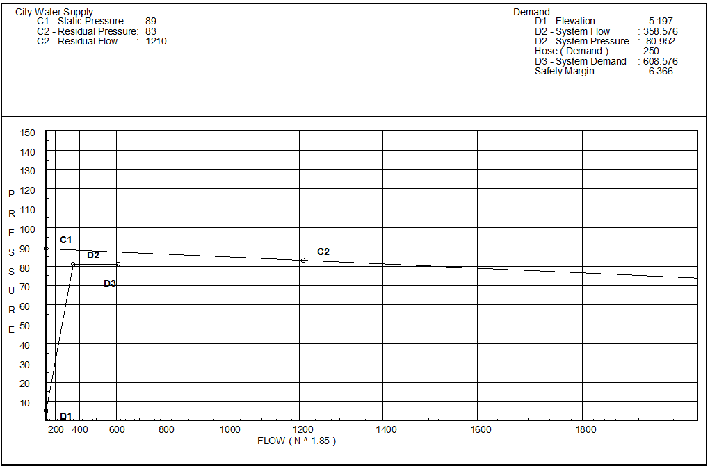
City Supply Only

This graph shows two curves, the City curve and the Demand curve.

The demand curve (in this case) has two demand points at the same pressure D2 and D3. This is because the exterior hose flow was added as an H250 flow. This allow this flow to be seen clearly. If the flow were entered as +250, the numerical result is the same, but the Demand curve is drawn directly from D1 to D2, where D2 takes the place of D3 and no D3 is shown.

See below for a key to the points and what they represent.

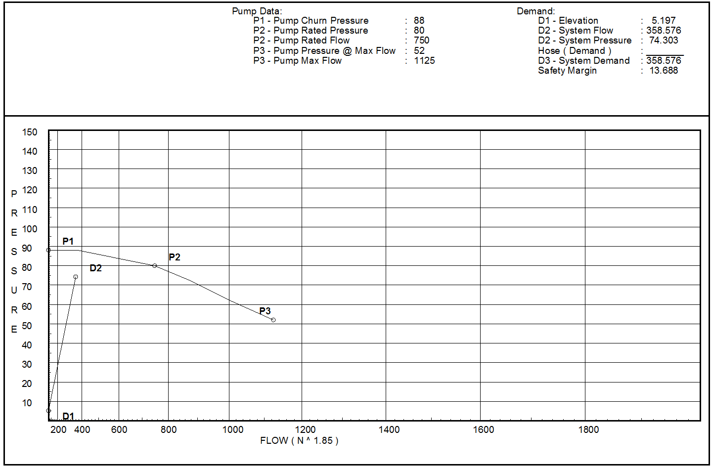
Pump Supply Only (No City Supply)

This graph shows two curves, the Pump curve and the Demand curve. The Pump curve is drawn using the Churn Pressure, the Rated Pressure and the Rated Flow. See below for a key to the points and what they represent.

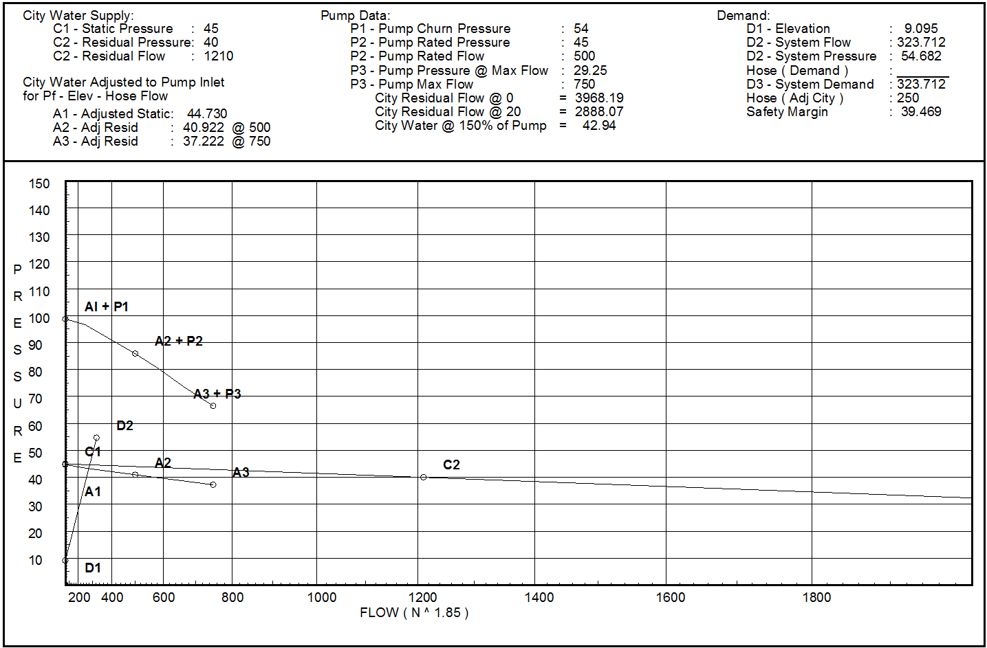
Pump and City Supply This graph shows four curves, the City curve, the Adjusted City curve, the combined Pump and Adjusted City curve and the Demand curve. The straight pump curve is omitted for clarity. The Adjusted City curve is calculated by flowing the various points along the pump curve from the Source back to the Pump Inlet. Any elevation changes, hose flows or friction losses are accounted for, usually resulting in a lower water pressure being available at the Pump Inlet versus the Source point.

The Adjusted City curve plus the Pump curve adds together these two curves, resulting in the water actually available.

See below for a key to the points and what they represent.

Key to Hydraulic Graph

The following table presents where the values on the graph come from, along with notes explaining in detail, if necessary. Some of these curves appear only if a pump is present, or a city supply is entered, or both.

These additional values appear on the Hydraulic Graph for information purposes:

Schematic Diagram

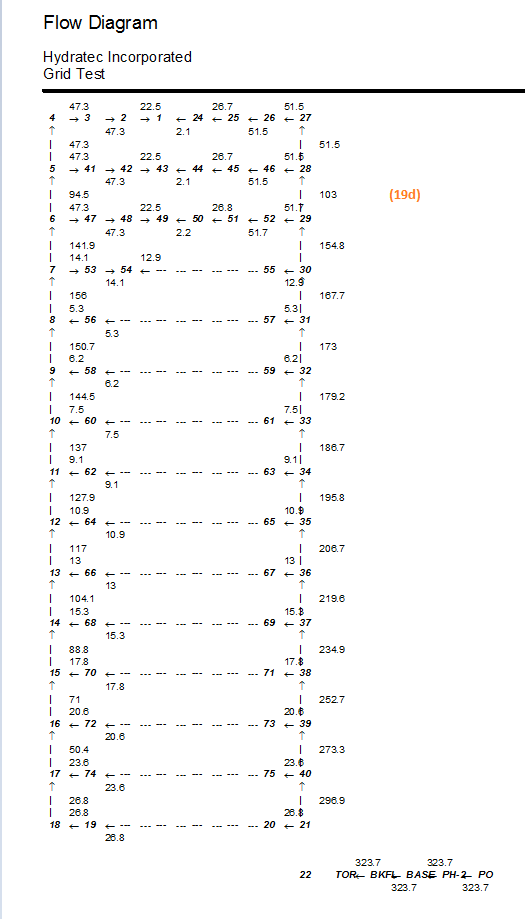
The Schematic Diagram is a graphical representation of the sprinkler system. It shows flows and the direction of flows. It is sometimes required with gridded systems.

For example, in the diagram at left, notice the reference nodes 4 and 3. The flow is listed as 47.3 (gal) and the flow goes from 4 to 3.

Also, at left notice reference node 1. It is fed 22.5 gal from the left and 2.1 gal from the right. This makes this the *split * head, and also the remote head on that line. Each gridded line in the remote area shows a split head.

This diagram can be built manually, automatically, or from HydraCALC-Sizer. HydraCAD can generate its own flow diagram in a drawing. For more information on creating this diagram, visit this topic: Schematic Diagram.

Fittings Used Summary

This report shows detailed information concerning the fittings that are used in the calculation. In the image below, note five fittings A, E, G, T and Zac, that were used somewhere in the calculation.

The Name of the fitting is printed after the Fitting Abbreviation.

After that appear the equivalent lengths that are assigned to all the sizes possible in HydraCALC, from ½” (12mm) to 24” (600mm). These are the ‘unadjusted’ equivalent lengths.

Certain NFPA standards require that the fittings lengths be adjusted based on the pipe type and c-factor used - a note to this effect appears at the bottom of this page.

These adjusted lengths are used on the hydraulic calculation sheets (later in this chapter). This part of the report is useful in that it shows what the equivalent lengths were before those adjustments.

The Zac fitting s values are based on a loss curve as opposed to a table, hence the note next to it.

Note - you can change the fitting abbreviation, the name and the values of the equivalent lengths by using the Alter Pipe and Fittings tool.

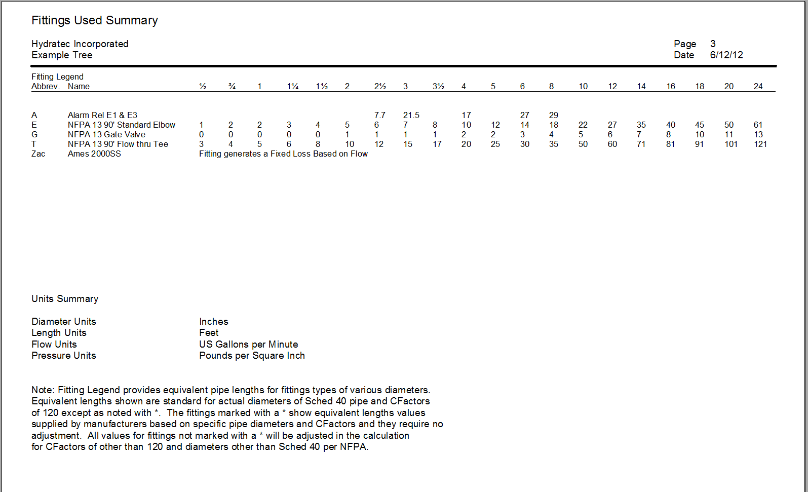
The units used in the calculation are stated in the Units Summary, below the Fitting Legend.

Flow Summary (Supply and Node Analysis Sheet)

This report lists all supply sources and nodes for the calculation.

The Supply Analysis shows both a pump source and a city source, if present. These are defined via the Water Source command.

The Available Pressure, Total Demand and Required Pressure columns are filled out for both pump and city sources.

Static and Residual pressures and residual Flow are displayed for city sources.

A pump, if used, does not record a static and residual pressure, instead that information is displayed on the Hydraulic Graph.

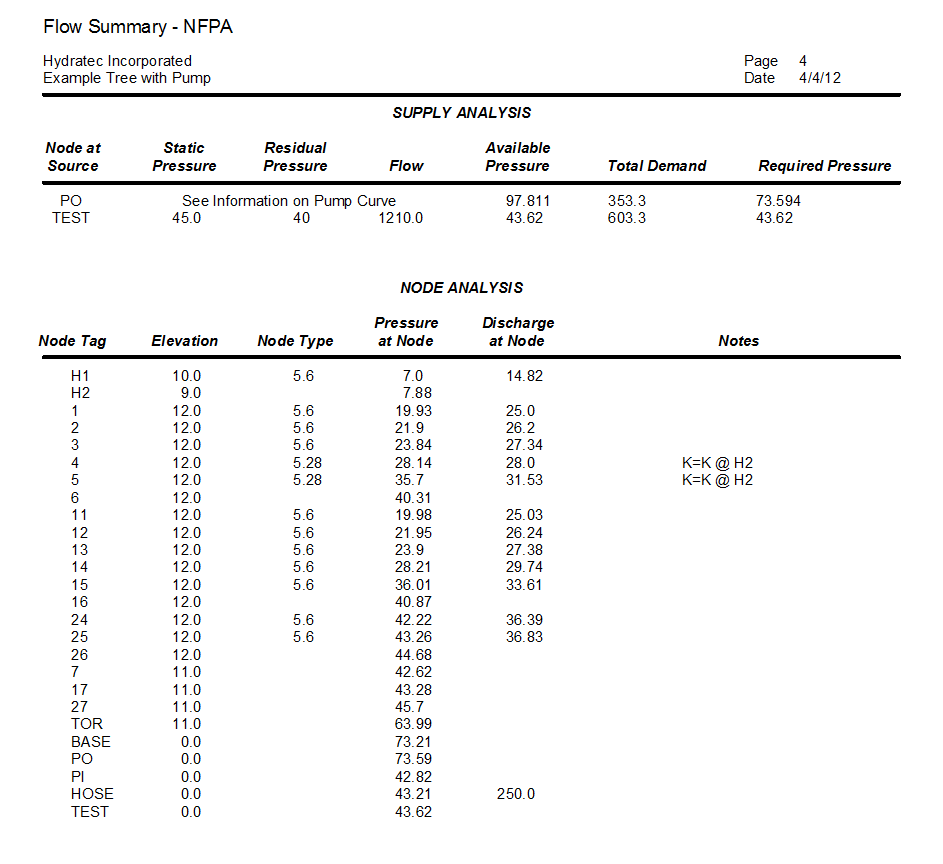
The Node Analysis lists all the nodes in the calculation. Elevations are listed for each node. The Node Type lists K-Factors added at the node point. The Pressure at Node is the pressure at that node, and the Discharge at Node is the flow calculated at the node. Hose flows appear in this column - note the 250.0 at node HOSE.

The Notes column is used for various information. The most common one concerns Equivalent K-Factors. Nodes 4 and 5, above, list a note K=K @ H2 . This mean the k-factor used at both nodes resulted from the k-factor generated at node H2.

Hydraulic Calculation Sheets

The Hydraulic Calculation Sheets are, perhaps, the most iconic of the reports. There are many numbers and codes on this report, so explaining it will require a few pages. The item numbers in the table correspond to the item numbers found in NFPA13 for this particular report. Certain items are added by HydraCALC for clarity when a pump is involved. These follow the required items.

Hazen Williams Calculation with or without a Pump

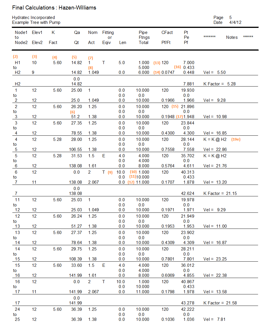
Hazen Williams Calculation with a Pump

Looking at the printout above, we can see the following:

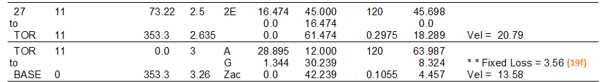
The System Demand at the pump outlet is 77.154 (psi)

The Safety Margin is 20.657

The Continuation Pressure (the safety margin plus the demand at the pump outlet) is 97.811. This item is something of an accounting measure, to show consistency as numbers are carried forward

The Pressure at Pump Outlet is simply the Continuation Pressure carried down to the pump section

The Pressure From Pump Curve shows -54.991. This is listed as a negative because it removes that much pressure from the demand on the city supply

The Pressure at Pump Inlet (42.820) is what is needed from the city supply at the pump inlet. If you follow that 42.820 back to the test point, you will end up at the 43.621 psi that is ultimately required from the city supply, after accounting for friction loss, elevation changes and valve and fitting losses.

Velocity Pressure Calculations

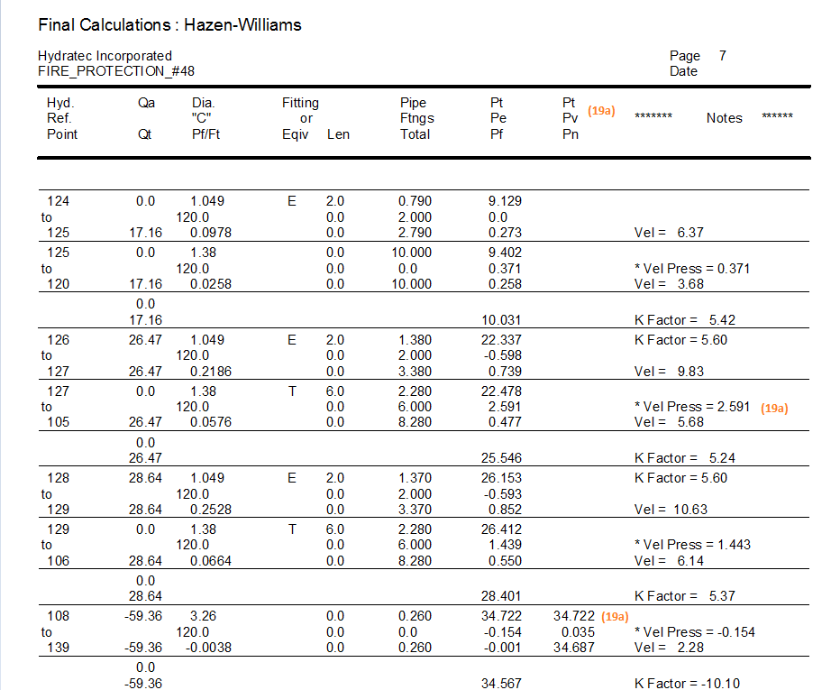
Velocity Pressure calculations have additional information, as needed. Some items in the report have been moved around to make room for the required column.

Darcy-Weisbach Calculations

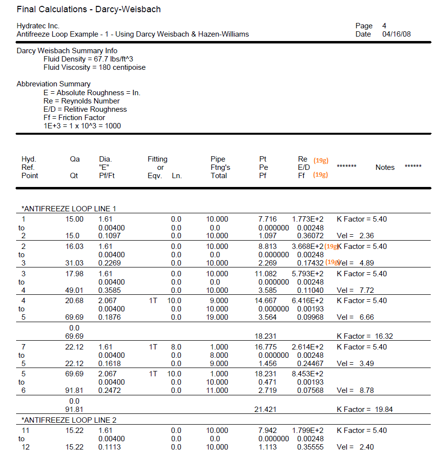
Darcy-Weisbach Calculations use different formulas than Hazen-Williams.

Additional information is included in the printout.

Auto Peaking Summary

NFPA requires peaking information if a computer program performed the peaking. The following report contains that information.

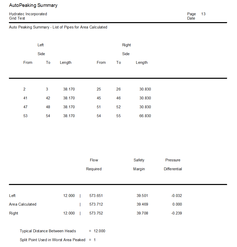
This report tells the user where the remote area is to be found in a gridded system. The List of Pipes for Area Calculated section reports where the remote area ended up after it was shifted automatically in the calculation. This is so the user can mark the remote area properly on their plan. The designations Left Side and Right Side are somewhat arbitrary, as they correspond to the L and R markers used in the setting up of the gridded calculation, not necessarily the physical orientation of the system on paper . L and R markers are explained in Tutorial #5 Calculating a Grid.

In the report above, the distance between reference points 2 and 3 is listed at 38.170 (feet). In this example, 2 is the branch line connection at the cross main and 3 is the first flowing head in the remote area. The other side is 30.830 ft. The fourth line, right side, from 54 to 55 is 66.830 ft due to that line having less flowing heads operating.

The next section of this report shows the demands associated with the remote area. The most remote area is the one listed as AREA CALCULATED. This area is the one referenced in the List of Pipes for Area Calculated. The Flow Required and Safety Margin are reported for this location.

The LEFT listing reports on the demands of the area if shifted one head left, at the distance seen (12.000). The one head RIGHT listing is also reported. These directions are consistent with the note above. If the remote area calculation had to move the remote area more than one head in a given direction, you will see multiple LEFT entries, each one one head further along the grid line, until the pressure starts to drop, and the peak is found.

The Typical Distance Between Heads is reported. The Split Point Used in Area Calculated refers to the reference point name designated to the most remote head.